The fourth step in a simulation study is to conduct simulation experiments with the model. Simulation is basically an application of the scientific method. In simulation, one begins with a theory of why certain design rules or management strategies are better than others. Based on these theories the designer develops a hypothesis which he tests through simulation. Based on the results of the simulation the designer draws conclusions about the validity of his hypothesis. In a simulation experiment there are input variables defining the model which are independent and may be manipulated or varied. The effects of this manipulation on other dependent or response variables are measured and correlated.
In some simulation experiments we are interested in the steady-state behavior of the model. Steady-state behavior does not mean that the simulation produces a steady outcome, but rather the distribution or statistical variation in outcome does not change over time. For example, a distribution warehouse may ship between 200 and 220 parts per hour under normal operating conditions. For many simulations we may only be interested in a particular time period, such as a specific day of the week. For these studies, the simulation may never reach a steady state.
As with any experiment involving a system with random characteristics, the results of the simulation will also be random in nature. The results of a single simulation run represent only one of several possible outcomes. This requires that multiple replications be run to test the reproducibility of the results. Otherwise, a decision might be made based on a fluke outcome, or at least an outcome not representative of what would normally be expected. Since simulation utilizes a pseudo-random number generator for generating random numbers, running the simulation multiple times simply reproduces the same sample. In order to get an independent sample, the starting seed value for each random stream must be different for each replication, ensuring that the random numbers generated from replication to replication are independent.
Depending on the degree of precision required in the output, it may be desirable to determine a confidence interval for the output. A confidence interval is a range within which we can have a certain level of confidence that the true mean falls. For a given confidence level or probability, say .90 or 90%, a confidence interval for the average utilization of a resource might be determined to be between 75.5 and 80.8%. We would then be able to say that there is a .90 probability that the true mean utilization of the modeled resource (not of the actual resource) lies between 75.5 and 80.8%.
Fortunately,
As part of setting up the simulation experiment, one must decide what type of simulation to run. Simulations are usually distinguished as being one of two types: terminating or non-terminating. The difference between the two has to do with whether we are interested in the behavior of the system over a particular period of time or in the steady-state behavior of the system. It has nothing to do, necessarily, with whether the system itself terminates or is ongoing. The decision to perform a terminating or non-terminating simulation has less to do with the nature of the system than it does with the behavior of interest.
A terminating simulation is one in which the simulation starts at a defined state or time and ends when it reaches some other defined state or time. An initial state might be the number of parts in the system at the beginning of a work day. A terminating state or event might be when a particular number of jobs have been completed. Consider, for example, an aerospace manufacturer that receives an order to manufacture 200 airplanes of a particular model. The company might be interested in knowing how long it will take to produce the aircraft along with existing workloads. The simulation run starts with the system empty and is terminated when the 200th plane is completed since that covers the period of interest. A point in time which would bring a terminating simulation to an end might be the closing of shop at the end of a business day, or the completion of a weekly or monthly production period. It may be known, for example, that a production schedule for a particular item changes weekly. At the end of each 40 hour cycle, the system is “emptied” and a new production cycle begins. In this situation, a terminating simulation would be run in which the simulation run length would be 40 hours.
Terminating simulations are not intended to measure the steady-state behavior of a system. In a terminating simulation, average measures are of little meaning. Since a terminating simulation always contains transient periods that are part of the analysis, utilization figures have the most meaning if reported for successive time intervals during the simulation.
A non-terminating or steady-state simulation is one in which the steady-state behavior of the system is being analyzed. A non-terminating simulation does not mean that the simulation never ends, nor does it mean that the system being simulated has no eventual termination. It only means that the simulation could theoretically go on indefinitely with no statistical change in behavior. For non-terminating simulations, the modeler must determine a suitable length of time to run the model.
Experiments involving terminating simulations are usually conducted by making several simulation runs, or replications, of the period of interest using a different random seed for each run. This procedure enables statistically independent and unbiased observations to be made on the system response over the period simulated. Statistics are often gathered on performance measures for successive intervals of time during the period.
For terminating simulations, we are usually interested in final production counts and changing patterns of behavior over time rather than the overall average behavior. It would be absurd, for example, to conclude that because two technicians are busy only an average of 40% during the day that only one technician is needed. This average measure reveals nothing about the utilization of the technicians during peak periods of the day. A more detailed report of waiting times during the entire work day may reveal that three technicians are needed to handle peak periods, whereas only one technician is necessary during off-peak hours. In this regard, Hoover and Perry (1990) note:
It is often suggested in the simulation literature that an overall performance be accumulated over the course of each replication of the simulation, ignoring the behavior of the systems at intermediate points in the simulation. We believe this is too simple an approach to collecting statistics when simulating a terminating system. It reminds us of the statistician who had his head in the refrigerator and feet in the oven, commenting that on the average he was quite comfortable.
For terminating simulations, the three important questions to answer in running the experiment are:
Many systems operate on a daily cycle, or, if a pattern occurs over a weeks time, the cycle is weekly. Some cycles may vary monthly or even annually. Cycles need not be repeating to be considered a cycle. Airlines, for example, may be interested in the start-up period of production during the introduction of a new airport which is a one-time occurrence.
The number of replications should be determined by the precision required for the output. If only a rough estimate of performance is being sought, three to five replications are sufficient. For greater precision, more replications should be made until a confidence interval with which you feel comfortable is achieved.
The issues associated with generating meaningful output statistics for terminating simulations are somewhat different that those associated with generating statistics for non-terminating systems. In steady-state simulations, we must deal with the following issues:
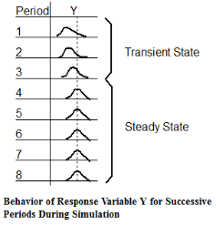
Determining the Warm-up Period In a steady-state simulation, we are interested in the steady-state behavior of the model. Since a model starts out empty, it usually takes some time before it reaches steady-state. In a steady-state condition, the response variables in the system (e.g., processing rates, utilization, etc.) exhibit statistical regularity (i.e., the distribution of these variables are approximately the same from one time period to the next). The following figure illustrates the typical behavior of a response variable, Y, as the simulation progresses through N periods of a simulation.
The time that it takes to reach steady-state is a function of the activity times and the amount of activity taking place. For some models, steady-state might be reached in a matter of a few hours of simulation time. For other models it may take several hundred hours to reach steady-state. In modeling steady-state behavior we have the problem of determining when a model reaches steady-state. This start-up period is usually referred to as the warm-up period. We want to wait until after the warm-up period before we start gathering any statistics. This way we eliminate any bias due to observations taken during the transient state of the model.
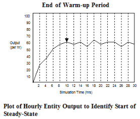
While several methods have been presented for determining warm-up time (Law and Kelton, 1991), the easiest and most straightforward approach, although not necessarily the most reliable, is to run a preliminary simulation of the system, preferably with several (3 to 5) replications, and observe at what time the system reaches statistical stability. The length of each replication should be relatively long and allow even rarely occurring events, such as infrequent downtimes, to occur at least two or three times. To determine a satisfactory warm-up period using this method, one or more key response variables should be monitored by period over time, like the average number of entities in a queue or the average utilization of a resource. This approach assumes that the mean value of the monitored response variable is the primary indicator of convergence rather than the variance, which often appears to be the case. If possible, it is preferable to reset the response variable after each period rather than track the cumulative value of the variable, since cumulative plots tend to average out instability in data. Once these variables begin to exhibit steady-state, we can add a 20% to 30% safety factor and be reasonably safe in using that period as the warm-up period. This approach is simple, conservative and usually satisfactory. Remember, the danger is in underestimating the warm-up period, not overestimating it. Relatively little time and expense is needed to run the warm-up period longer than actually required. The following figure illustrates the average number of entities processed each hour for several replications. Since statistical stability is reached at about 10 hours, 12 to 15 hours is probably a safe warm-up period to use for the simulation.
Obtaining Sample Observations In a terminating simulation, sample observations are made by simply running multiple replications. For steady-state simulations, we have several options for obtaining sample observations. Two widely used approaches are running multiple replications and interval batching. The method supported in
Running multiple replications for non-terminating simulations is very similar to running terminating simulations. The only difference is that (1) the initial warm-up period must be determined, and (2) an appropriate run length must be determined. Once the replications are made, confidence intervals can be computed as described earlier in this chapter. One advantage of running independent replications is that samples are independent. On the negative side, running through the warm-up phase for each replication slightly extends the length of time to perform the replications. Furthermore, there is a possibility that the length of the warm-up period is underestimated, causing biased results.
Interval batching (also referred to as the batch means technique) is a method in which a single, long run is made with statistics being reset at specified time intervals. This allows statistics to be gathered for each time interval with a mean calculated for each interval batch. Since each interval is correlated to both the previous and the next intervals (called serial correlation or autocorrelation), the batches are not completely independent. The way to gain greater independence is to use large batch sizes and to use the mean values for each batch. When using interval batching, confidence interval calculations can be performed. The number of batch intervals to create should be at least 5 to 10 and possibly more depending on the desired confidence interval.
Determining Run Length Determining run length for terminating simulations is quite simple since there is a natural event or time point that defines it for us. Determining the run length for a steady-state simulation is more difficult since the simulation can be run indefinitely. The benefit of this, however, is that we can produce good representative samples. Obviously, running extremely long simulations is impractical, so the issue is to determine an appropriate run length that ensures a sufficiently representative sample of the steady-state response of the system is taken.
The recommended length of the simulation run for a steady-state simulation is dependent upon (1) the interval between the least frequently occurring event and (2) the type of sampling method (replication or interval batching) used. If running independent replications, it is usually a good idea to run the simulation enough times to let every type of event (including rare ones) happen at least a few times if not several hundred. Remember, the longer the model is run, the more confident you can become that the results represent a steady-state behavior. If collecting batch mean observations, it is recommended that run times be as large as possible to include at least 1000 occurrences of each type of event (Thesen and Travis, 1992).
Simulations are often performed to compare two or more alternative designs. This comparison may be based on one or more decision variables such as buffer capacity, work schedule, resource availability, etc. Comparing alternative designs requires careful analysis to ensure that differences being observed are attributable to actual differences in performance and not to statistical variation. This is where running multiple replications may again be helpful. Suppose, for example, that method A for deploying resources yields a throughput of 100 entities for a given time period while method B results in 110 entities for the same time period. Is it valid to conclude that method B is better than method A, or might additional replications actually lead the opposite conclusion?
Evaluating alternative configurations or operating policies can sometimes be performed by comparing the average result of several replications. Where outcomes are close or where the decision requires greater precision, a method referred to as hypothesis testing should be used. In hypothesis testing, first a hypothesis is formulated (e.g., that methods A and B both result in the same throughput) and then a test is made to see whether the results of the simulation lead us to reject the hypothesis. The outcome of the simulation runs may cause us to reject the hypothesis that methods A and B both result in equal throughput capabilities and conclude that the throughput does indeed depend on which method is used.
Sometimes there may be insufficient evidence to reject the stated hypothesis and thus the analysis proves to be inconclusive. This failure to obtain sufficient evidence to reject the hypothesis may be due to the fact that there really is no difference in performance, or it may be a result of the variance in the observed outcomes being too high given the number of replications to be conclusive. At this point, either additional (perhaps time consuming) replications may be run or one of several variance reduction techniques might be employed (see Law and Kelton, 1991).
In simulation experiments we are often interested in finding out how different input variable settings impact the response of the system. Rather than run hundreds of experiments for every possible variable setting, experimental design techniques can be used as a “short-cut” to finding those input variables of greatest significance. Using experimental-design terminology, input variables are referred to as factors, and the output measures are referred to as responses. Once the response of interest has been identified and the factors that are suspected of having an influence on this response defined, we can use a factorial design method which prescribes how many runs to make and what level or value to be used for each factor. As in all simulation experiments, it is still desirable to run multiple replications for each factor level and use confidence intervals to assess the statistical significance of the results.
One's natural inclination when experimenting with multiple factors is to test the impact that each individual factor has on system response. This is a simple and straightforward approach, but it gives the experimenter no knowledge of how factors interact with each other. It should be obvious that experimenting with two or more factors together can affect system response differently than experimenting with only one factor at a time and keeping all other factors the same.
One type of experiment that looks at the combined effect of multiple factors on system response is referred to as a two-level, full-factorial design. In this type of experiment, we simply define a high and low level setting for each factor and, since it is a full-factorial experiment, we try every combination of factor settings. This means that if there are five factors and we are testing two different levels for each factor, we would test each of the 25 = 32 possible combinations of high and low factor levels. For factors that have no range of values from which a high and low can be chosen, the high and low levels are arbitrarily selected. For example, if one of the factors being investigated is an operating policy for doing work (e.g., first come, first served; or last come, last served), we arbitrarily select one of the alternative policies as the high level setting and a different one as the low level setting.
For experiments in which a large number of factors are being considered, a two-level full-factorial design would result in an extremely large number of combinations to test. In this type of situation, a fractional-factorial design is used to strategically select a subset of combinations to test in order to “screen out” factors with little or no impact on system performance. With the remaining reduced number of factors, more detailed experimentation such as a full-factorial experiment can be conducted in a more manageable fashion.
After fractional-factorial experiments and even two-level full-factorial experiments have been performed to identify the most significant factor level combinations, it is often desirable to conduct more detailed experiments, perhaps over the entire range of values, for those factors that have been identified as being the most significant. This provides more precise information for making decisions regarding the best factor values or variable settings for the system. For a more concise explanation of the use of factorial design in simulation experimentation see Law and Kelton (1991).
One of the most valuable characteristics of simulation is the ability to reproduce and randomize replications of a particular model. Simulation allows probabilistic phenomena within a system to be controlled or randomized as desired for conducting controlled experiments. This control is made available through the use of random streams.
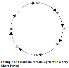
A stream is a sequence of independently cycling, unique random numbers uniformly distributed between 0 and 1 (see the figure on next page). Random number streams are used to generate additional random numbers from other probability distributions (Normal, Beta, Gamma). After sequencing through all of the random numbers in the cycle, the cycle starts over again with the same sequence. The length of the cycle before it repeats is called the cycle period and is usually very long.
A random stream is generated using a random number generator or equation. The random number generator begins with an initial seed value after which, each successive value uses the previous value as input to the generator. Each stream used in a simulation has its own independent seed and tracks its own values for subsequent input to the generator. Where the sequence begins in the cycle depends on the initial seed value used by the generator.
Any time a particular number seeds a stream, the same sequence of values will be repeated every time the same seed is used to initialize the stream. This means that various elements within a model can be held constant with respect to their performance while other elements vary freely. Simply specify one random number stream for one set of activities and another random number stream for all other activities.
Because the same seed produces the same sequence of values every time it is used, completely independent functions within a model must have their own streams from the start. For example, arrival distributions should generally have a random number stream used nowhere else in the entire model. That way, activities added to a model that sample from a random number stream will not inadvertently alter the arrival pattern because they do not affect the sample values generated from the arrival distribution.
To show an example of how multiple streams can be useful, consider two copy machines, Copy1 and Copy2, which go down approximately every 4 hours for servicing. To model this, the frequency or time between failures is defined by a normal distribution with a mean value of 240 minutes and a standard deviation of 15 minutes, N(240,15). The time to repair is 10 minutes. If no stream is specified in the normal distribution, the same stream will be used to generate sample values for both machines. So, if the next two numbers in the stream number are .21837 and .86469, Copy1 will get a sample value from the normal distribution that is different from Copy2. Therefore, the two machines will go down at different times.
Suppose, however, that the resource servicing the machines must service them both at the same time, so we would like to have the machines go down at the same time. Using the same stream to determine both downtimes will not bring them down at the same time, because a different random number will be returned from the stream with each call to generate a random normal variate. Using two different streams, each dedicated to a machine's downtime and each having the same initial seed, will ensure that both machines go down at the same time every time. The two streams have the same starting seed value so they will produce exactly the same sequence of random numbers.

|
© 2012 ProModel Corporation • 556 East Technology Avenue • Orem, UT 84097 • Support: 888-776-6633 • www.promodel.com |